
Contents
Comparing Feedback and Feedforward Controls
The main differences between feedback and feedforward control are:
- feedforward controller calculates the control without measurement of the process output (control variable).
- feedforward works solely based on the priory knowledge (model) of process/disturbance. Since the model is never 100% accurate, the contribution of feedforward controller is always approximate.
- Unlike feedforward, feedback is error-driven. Hence, feedback control usually acts much slower than feedforward control since it needs to wait for generation of error.
- Application of feedforward control is limited to known/predictable/measureable disturbances or commands.
- designing a feedforward controller often takes much more effort compared to feedback controller design.
Two Feedforward Control Structures for Disturbance Rejection
In this article we study the application of feedforward control to enhance the disturbance rejection and command following capability of feedback control systems. For this purpose, consider Fig. 1 where \(G_u(s)\) is the transfer function model of plant and \(G_c(s)\) is the transfer function of controller (which is, for example, a proportional controller or a PI controller).
Although this system is widely used in many real world applications, it has some limitations. First, it is known that in this system the dynamics of setpoint tracking is different with the dynamics of disturbance rejection. It means that in general it is not possible to design the controller such that the response of the feedback control system to step changes in both setpoint and disturbance be satisfactory at the same time.
In other words, when the transient response to a step change in setpoint is satisfactory, it is very likely not satisfactory to a step change in disturbance, and vice versa. Considering the fact that in today’s real world applications the priority is usually given to setpoint tracking, the disturbance rejection response of the feedback control system is usually not really satisfactory. That is why techniques like Ziegler-Nichols methods which only try to improve the response of the feedback control system to step disturbance are not suitable for today applications.
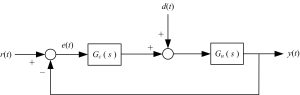
Figure 1: block diagram of the feedback control system
The other drawback of the feedback control system of Fig. 1 for disturbance rejection purposes is that in this system first the disturbance should corrupt the output of plant and then the controller begins compensation for it. In other words, the reaction of this closed loop system to the input disturbance is slow. One possible solution to all of the above mentioned drawbacks is to combine the feedback control with feedforward control. The block diagram of two well-known feedback-feedforward control systems are shown in Figures 2 and 3.
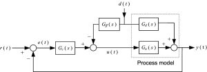
Figure 2: the first strategy for feedforward control
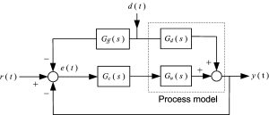
Figure 3: the second strategy for feedforward control
In these figures \(G_{ff}(s)\) shows the transfer function of the feedforward controller to be designed. Note that in Figure 1 the disturbance enters directly into the input of plant, while in the feedforward control of Figures 2 and 3 the disturbance enters into plant from a different and separate path. So, not every given closed loop system in the form of Figure 1 can be upgraded by adding the feedforward control system. In the following we elaborate on designing the feedforward control in Figures 2 and 3, but before that we need to learn more about the notion of “disturbance”.
What is Disturbance?
- Disturbance is modeled as an input signal which can enter to different points of the control system.
- Disturbance is often (but not always) is a low-frequency signal. It meas that the its power spectral density (PSD) or Fourier transform is mostly centered around the origin.
- Disturbance is (ideally) uncorrelated with the setpint (command) input.
- Disturbance may not be a real external signal, that is, it might be an exogenous input used for modelling some error.
Prerequisite For Feedforward Control: Measurable Disturbance
The key prerequisite for designing a feedforward control system is that the input disturbance must be measurable. Although it may look weird at the first glimpse, the disturbance can really be measured in many real world applications. One general problem of this kind appears in controlling a two-input one-output plant when one of the inputs cannot be changed by the user but it can be measured.
For instance, consider the room temperature control problem as shown in Figure 4 where two heaters are placed in a room and it is expected that together they provide the power needed to warm up the room and regulate its temperature at the desired value.
As seen in Fig. 4, it is assumed that one of these heaters is connected to a solar panel which is not a reliable power source. It means that the power delivered by the solar panel to the corresponding heater is out of our control and can change if e.g. a piece of cloud casts a shadow on it.
Hence, although the first heater has a contribution to the room temperature, the amount of energy delivered by it is neither exactly predictable nor can be adjusted. On the other hand, the other heater is connected to the grid by means of a PWM-controlled switch. Hence, this heater can always deliver 0 to 100% of its nominal power by changing the duty cycle of PWM.
To sum up, this plant has two inputs; one of them is the disturbance input which is equal to the power generated by the heater connected to the solar panel, and the other one is the control input which is equal to the power generated by the heater connected to the grid. The very important point is that in this plant the disturbance input can be measured very accurately by means of a power meter (i.e., it is a measurable disturbance as required for feedforward control design).
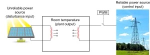
Figure 4: room temperature control problem, an example of measurable disturbance
As another example, consider the sewage pH control problem where the sewage enters into a tank and a chemical solution with a constant pH and controllable flow is also added to the liquid in tank to regulate the pH of the resulting solution to the desired value. The liquid with regulated pH continuously goes out of the tank for further processing.
Here, again we have a two-input one-output process (input 1: sewage flow, input 2: chemical solution flow, output: pH of the liquid in tank) where one of inputs is out of our control and can be considered as a disturbance input and the other one can be considered as the control input. Obviously, in this example the sewage flow (input disturbance) can be measured accurately which is essential for feedforward control design.
The other limitation of feedforward control is that the dynamics of measureable disturbance (i.e. the transfer function \(G_d\) in Figures 2 and 3) must be known very accurately (sometimes in the control literature \(G_d\) is called the disturbance model, which must be known).
In fact, successful application of feedforward control strategy strongly depends on the accuracy of this part of model. Note that unlike \(G_d\), \(G_u\) does not need to be identified very accurately since it is located in the feedback loop and we know from the control theory that any appropriately design feedback control system has the property of reducing the sensitivity of closed loop transfer function to the open loop transfer function.
How To Design a Feedforward Control System?
First consider Fig. 2 and assume that the transfer functions \(G_d(s)\) and \(G_u(s)\) are known. The design problem is to calculate the unknown transfer functions \(G_c\) and \(G_{ff}\) such that setpoint tracking and disturbance rejection are done well.
The very important point is that these feedback and feedforward controllers can be designed independently. So, it doesn’t matter which one of \(G_c\) and \(G_{ff}\) is designed first. It is easy (for example, by using Mason’s formula) to show that here we have
\[Y(s)=\frac{G_d-G_{ff}G_u}{1+G_cG_u}D(s)+\frac{G_cG_u}{1+G_cG_u}R(s)\]
Ideally, we need the first term in the right hand side of the above equation be equal to zero. For this purpose we can simply calculate the feedforward control law, \(G_{ff}\), from the following equation
\[G_{ff}=\frac{G_d}{G_u}\]
Recall that only causal systems can be realized online (in real time). The transfer function obtained for \(G_{ff}\) in the above equation is causal and can be used in real time applications if and only if the degree of its numerator is larger than or equal to the degree of its denominator. For this purpose the relative degree of the disturbance model, \(G_d\) must be smaller than or equal to the relative degree of the plant transfer function model, \(G_u\) (the relative degree is defined as the difference between the degree of polynomial at the numerator and the polynomial at the denominator of a transfer function).
In order to design \(G_c\), neglect the feedforward controller and consider Fig. 1. In this figure calculate \(G_c\) such that the feedback control system has a satisfactory setpoint tracking characteristics. For example, \(G_c\) can be considered as a PI controller and its parameters can be tuned using one of the methods presented here.
Numerical Feedforward Control Design Example
In Fig. 5 the results of a numerical simulation are presented. As it is seen, here it is assumed that \(G_u=\frac{1}{s+1}\) and \(G_d=\frac{0.5}{0.7s+1}\) which concludes that the transfer function of feedforward control system equals \(G_{ff}=\frac{G_d}{G_u}=\frac{0.5s+0.5}{0.7s+1}\). But, we learned that in real world applications we never know the exact transfer function model of process and disturbance, that is our knowledge of \(G_u\) and \(G_d\) is limited and accompanied with some error.
That is why in Fig. 5 it is assumed that \(G_{ff}(s)=\frac{0.45s+0.55}{0.8s+0.9}\), whose coefficients are slightly different with the \(G_{ff}(s)\) calculated above. Note that the values considered in Fig. 5 for the coefficients of \(G_{ff}(s)\) are chosen randomly and infinity many other values work as well. Simulation results of a feedback control systems, one with and the other one without feedforward control, are shown in Fig. 5.
As it can be seen, even the feedforward controller with perturbed coefficients leads to a much better result compared to the case there is no feedforward control. In this simulation the transfer function of PI controller, which is tuned using the Simulink auto-tuner, is \(1.44+4.45/s\).
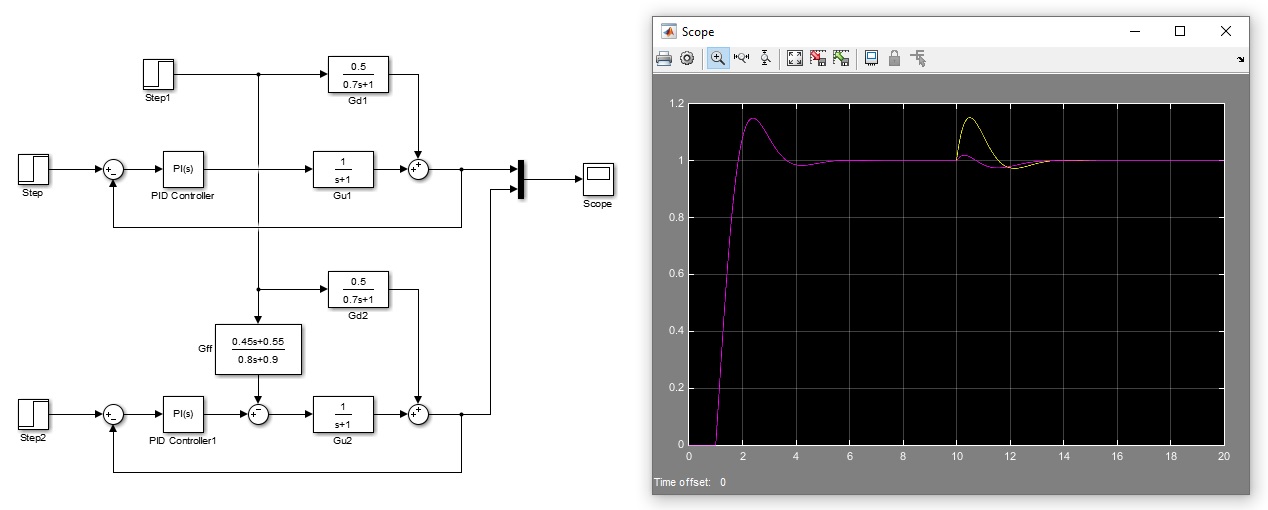
Figure 5: Simulation results of two feedback control systems (with and without feedforward control)
You can find amazing films on tuning PID/PI controllers here.
Written by Farshad Merrikh-Bayat