
Contents
What Is PI Controller?
PI controller is a special case of PID – Proportional Integral Derivative – which is a linear controller with three tuning parameters. The derivative term in PID is barely used in real world applications, that is why the controller is usually in the form of a PI controller. In fact, PI controller is used more than any other process controller and in almost any industrial application like water level control, temperature control, flow control, dc motor speed control, ac motor speed control, etc. there exists a PI controller.
It is a well-known fact that PI controller is sufficient to control stable processes whose step response is s-shaped without a considerable time delay or their Nyquist plot is located only in the first and fourth region of the complex plane. It is also known that PI controller is not a good choice and considering derivative term is useful when the process is high order or it has some poles with very different time constants.
7 Methods to Tune the Parameters of a PI Controller
In the following we review 6 methods for PID controller tuning which take into account the proportional controller and PI controller as a special case. Historically, the first general P/PI/PID loop tuning rules were proposed by Ziegler and Nichols in 1942, which are currently known as Ziegler Nichols method for PID tuning method. After that, enormous PI/PID tuning methods were developed by other researchers. Clearly, not all of these methods have the same performance and popularity. The following PI/PID tuning guide is carefully prepared to be concise yet useful. “PID autotune” is another important subject in the field of PID loop tuning which is discussed in the following.
Finally note that this article is about one degree of freedom (1DOF) feedback control system. For more information on related techniques see the articles on feedforward control and open loop control system.
Method 1: Ziegler Nichols (ZN) step response method (Obsolete!)
- Can be used for P controller, PI controller, and PID controller tuning (but not PD controller tuning)
- Only step response of the open loop system is required for P/PI/PID tuning (advantage)
- response of the open loop system to step input can be oscillatory damped or in the form of a s shaped curve. The method can also be used for P controller/PI controller/PID controller design for an integrating process (DC motor and water level control are examples of integrating process).
- The purpose of controller design is to arrive at a closed loop system with a decay ratio of ¼ in response to a step disturbance which enters to the process input. Note that only disturbance rejection (but not setpoint tracking) is under consideration in this method.
- The first big advantage of ZN step response method is that it needs very little information about the process. The second big advantage is that the P controller/PI controller/PID controller tuning formulas are summarized in user-friendly tables.
- The main disadvantage of this ZN PID/PI tuning method is that it usually leads to large overshoots in the response of closed loop system, especially when setpoint tracking is under consideration. The reason is the damping ratio of the resulting feedback system is very small (approximately 0.2) since the proportional gain is 2-3 times larger than its appropriate value. The other drawback is that there is no table for PD controller design, which is indeed barely used in real world applications.
- Caution: This PID/PI controller tuning method does not lead to acceptable results for today’s applications. Don’t use it, it is obsolete! There are much better methods (see Methods 3-6 below).
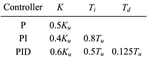
- Controller design algorithm: Draw the tangent line with maximum slope on the response of plant to the unit step input and determine parameters a and L (process delay) as shown in Figures 1 and 2 (which is a s shaped curve). Then calculate the P/PI/PID parameters from Table 1. The transfer function of PID controller is where and are the PID integral and derivative time, respectively.
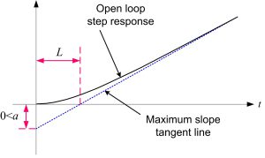
Fig. 1: response of an integrating process to step input
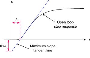
Fig. 2: step response of the open loop system in the form of an s shaped curve
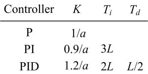
Table 1: P/PI/PID controller tuning using the Ziegler Nichols step response method
- Controller design example: Assume that the open loop process model is \(G(s)=\frac{1}{(s+1)^3}\). Response of the open loop system to step input together with the maximum slope tangent line are shown in Figure 3. From this figure the values of \(a\) and \(L\) are obtained equal to 0.218 and 0.860, respectively, and the parameters of controller are calculated as \(K=5.50,T_i=1.61\), and \(T_d=0.403\). Response of the closed loop system to the unit step command and unit step disturbance (which enters at t=50s to the process input) with this controller in the feedback loop is shown in Fig. 4.
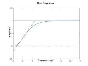
Fig. 3: response of the open loop control system to step input (in the form of an s shaped curve) and the tangent line with maximum slope
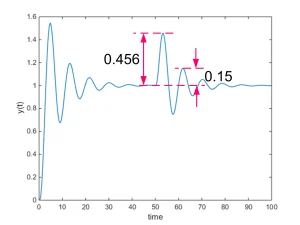
Fig. 4: response of the closed loop system to unit step (decay ratio of ~0.25 in step disturbance rejection is observed)
Method 2: Ziegler Nichols (ZN) frequency response method (Obsolete!)
- Can be used for P controller, PI controller, and PID tuning (but not PD controller tuning)
- Information of only one point on the Nyquist plot of the open loop system is required (advantage). This information can be obtained in two ways: relay feedback or proportional feedback. In both of these methods we put the series connection of process and a proportional controller or relay in a feedback loop and wait until stable oscillation appears at the output of process. The relay feedback method is more favorite since (hopefully!) oscillation begins automatically. For this reason, this method for Proportional Integral Derivative controller design is referred to as PID/PI auto tuning (or, autotuning). Note that a linear plant with relative degree equal to one or two can never generate stable oscillations when it is located in the forward path of a feedback loop in series with a proportional controller (the reason can be understood from the root locus method).
- The purpose of controller design is to arrive at a closed loop system with a decay ratio of ¼ in response to a step disturbance which enters to the input of plant. Note that only disturbance rejection (but not setpoint tracking) is under consideration.
- The advantages and disadvantages of this PID/PI controller design method are the same as ZN step response method. The additional drawback of this method is that in order to find the information of the certain point on the Nyquist plot of process, the feedback system must oscillate which may be harmful in real world applications. Note that ZN frequency response method usually leads to smaller overshoots in the step response of the closed loop compared to the previous ZN method.
- Caution: This PID/PI controller tuning method is obsolete since it does not lead to acceptable results for today’s applications. Don’t use it, it is obsolete! There are much better methods (see Methods 3-6 below).
- Controller design algorithm: put the process in a unity feedback loop in series with a relay as shown in Fig. 5 where , and is the standard signum function. Hopefully oscillation begins automatically! At steady state, the process output and input are in the form of a (pseudo) sinusoidal wave and rectangular wave, respectively. Denote the ratio of the amplitude of input to the amplitude of output at steady state as , and the period of oscillation at steady state as . Then the parameters of proportional controller, PI controller, and PID can be calculated from Table 2 where the controller transfer function is considered as .
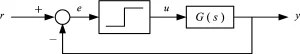
Fig. 5: relay feedback method
- Note that the ZN frequency response method actually moves the ultimate point on the Nyquist plot of plant (i.e. the point on the Nyquist plot which intersects the negative real axis) to -0.6-0.28j
- Controller design example: Assume that the open loop plant model is \(G(s)=\frac{1}{(s+1)^3}\). If we put this plant in the closed loop system of Figure 5 the system begins oscillation. The input and output of plant in this case will be as shown in Fig. 6. As it is seen, the phase difference between input and output of plant at steady state approximately equals to 180 degrees. The period of oscillation at steady state is \(T_u=3.68\) s, and we have \(K_u=0.1631\) (note that the corresponding exact values obtained from the Bode plot as shown in Fig. 6 are \(T_u=3.6110\) and \(K_u=0.123\)). Now, using Table 2 for PID controller design yields \(K=0.098,T_i=1.84\), and \(T_d=0.46\). Response of the feedback system to the unit step command and unit step disturbance (which enters at t=50s to the process input) with this controller in the feedback loop is shown in Fig. 8.
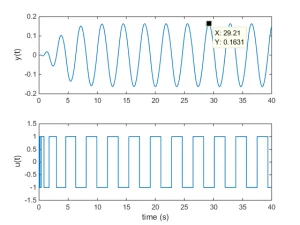
Fig. 6: stable oscillations using relay feedback method
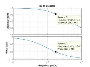
Fig. 7: Bode plot of the process model
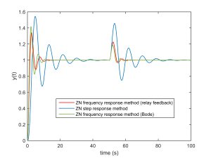
Fig. 8: response of the closed loop system to unit step command and unit step disturbance (which enters at the input of process at t=50 s)
Table 2: P/PI/PID controller tuning using the Ziegler Nichols frequency response method
Method 3: AMIGO PI controller tuning method (AMIGO: Approximate \(M_s\) -Constrained Integral Gain Optimization)
- This method can be used only for PI controller design either for an integrating process with transfer function \(G(s)=\frac{K_ve^{-sL}}{s}\) (which appears in e.g. level control of liquid in a tank) or a stable first order plus time delay (FOPTD) process with transfer function \(G(s)=\frac{K_pe^{-sL}}{1+sT}\) (which appears in e.g. temperature control). These two process models appear in many real world applications. Recall that more than 90% of the controllers currently in use in industries are PI controllers.
- The emphasis of this method is on disturbance rejection but the setpoint tracking is also satisfactory in most cases.
- This PI controller tuning method maximizes the integral gain subject to a constraint on the peak of the sensitivity function. We know that increasing the integral gain speeds up the closed loop system response but it also reduces the phase margin – PM – and gain margin – GM – and leads to larger overshoots in the response of the feedback system (recall that reducing the phase margin and gain margin is equivalent to increasing the peak of the sensitivity function). AMIGO method limits the peak of sensitivity function to \(M_s=1.4\) which means that the gain margin and phase margin of the feedback control system are at least equal to 3.5 and 45 degrees, respectively (recall that in real world applications usually a phase margin of about 45 to 60 degrees is desired). The graphical definition of PM, GM and \(M_s\) based on the Nyquist plot of the open loop system, which is denoted as \(L(s)=C(s)G(s)\), is depicted in Fig. 9.
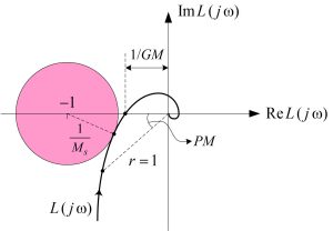
Fig. 9: graphical representation of PM, GM, and peak of the sensitivity function (\(M_s\))
- Controller design algorithm: Consider the transfer function of PI controller as \(C(s)=K\left(1+\frac{1}{sT_i}\right)\). If the stable plant model is in the form of a FOPTD transfer function then define \(K_v:=K_p/T\) and calculate the parameters of PI controller from the following equation s
\[K=\left\{
\begin{array}{ll}
\frac{0.35}{K_vL}-\frac{0.6}{K_p}, & L<T/6 \\
\frac{0.25T}{K_pL}, & T/6<L<T \\
\frac{0.1T}{K_pL}+\frac{0.15}{K_p}, & T<L
\end{array}
\right.\]
\[T_i=\left\{
\begin{array}{ll}
7L, & L<0.11T \\
0.8T, & 0.11T<L<T \\
0.3L+0.5T, & T<L
\end{array}
\right.\]
- Note that in order to find the FOPTD process model there is no need for exerting complicated system identification algorithms and such a plant model can be obtained from the step response of the process as shown in Figure 10.
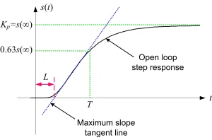
Fig. 10: finding FOPTD process model from the step response of process.
- For an integrating process, PI controller design can be done through the following equations
\[K=\frac{0.35}{K_vL}\]
\[T_i=7L\]
- Notice that the parameters of integrating process can be found with a simple experiment as shown in Fig. 11 and without the need for applying complicated system identification methods. For this purpose, apply the pulse \(p(t)\) as shown in Fig. 11 to plant and observe the response of plant, \(q(t)\), at output. Then draw the tangent line with maximum slope as shown in this figure and calculate the process velocity gain \(K_v\) and process delay \(L\) as detailed in Fig. 11. After that the parameters of PI controller can be calculated from the above equations.
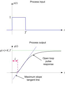
Fig. 11: identifying the parameters of integrating process model from the pulse response of plant
Method 4: CHR method for P/PI/PID loop tuning
- Can be used for P controller, PI controller, and PID tuning (but not PD controller tuning)
- There is no need to know the exact plant model. Only the response of the plant to step input is required for PID/PI controller tuning.
- Presenting PID/PI tuning guide in two separate tables; one for load disturbance rejection and the other one for setpoint tracking (recall that with the 1DOF feedback control system we cannot have good disturbance rejection and setpoint tracking at the same time, and the control system designer should determine the control priority in advance).
- In each table the control system designer can select the PID parameters (or PI controller parameters or the proportional controller gain) to arrive at a feedback control system with 0% or 20% overshoot in the closed loop step response.
- Controller design algorithm: Draw the tangent line with maximum slope to the step response of the process as shown in Figure 2, and determine the parameters a and L (system time delay), and T (system time constant). Consider the controller transfer function as and calculate the parameters from Table 3 for disturbance rejection and Table 4 for setpoint tracking.
- Note that unlike Ziegler Nichols methods the process time constant, T, also appears in one of the tables (see Table 4).
- Drawbacks of the CHR method: 1- very large overshoots in the setpoint tracking response when the controller is designed for disturbance rejection, 2- so sensitive to the plant model (the results are not satisfactory when the plant transfer function is not originally in the form of a FOPTD and such a model is obtained approximately)
Table 3: PID/P/PI controller tuning for load disturbance rejection using CHR method
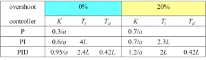
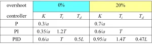
Table 4: PID/P/PI controller tuning for setpoint tracking using CHR method
Method 5: PI/PID tuning with pidtune function of Matlab
- pidtune function of Matlab is a very user-friendly method for PID/PI auto tuning.
- This controller design algorithm calculates the PD/PI/PID parameters such that at the desired gain crossover frequency the phase of the open loop system be equal to the desired value or gets as close as possible to it (crossover frequency is the frequency at which the magnitude of the open loop system equals one).
- Note that by adjusting the phase of the open loop system at the crossover frequency to an appropriate value we can adjust the phase margin to the desired value. Moreover, the crossover frequency approximately equals to the bandwidth of the closed loop system. So, in order to speed up the closed loop system response we can assign a larger value to the crossover frequency. Note that time constant of the step response of the closed loop system approximately equals to inverse of the crossover frequency.
- Predefined value for phase margin equals 60 deg. It is a very favorite value in many real world applications.
- Matlab automatically considers an appropriate value for crossover frequency if the user does not specify it.
- Transfer function of controller is considered in the parallel form, that is(see the article transfer function of PID for more information on this).
- It is a very high quality tuning method. Strongly recommended!
Method 6: PID/P/PD/PI controller tuning with Cohen Coon method
- Belongs to the category of analytic tuning methods (like internal model control – IMC).
- Controller tuning rules are obtained assuming that the plant model is in the form of a first order plus time delay (FOPTD) transfer function.
- The Cohen Coon method locates the dominant poles of the closed loop control system in complex plane with the aim of rejecting step disturbance with the decay ratio of 0.25 (note that the priority is given to disturbance rejection but not setpoint tracking, and limiting the decay ratio to 0.25 determines a region in complex plane).
- When designing a proportional controller or PD controller (also known as proportional derivative controller) the gains of controller are optimized such that the tracking error caused by step disturbance at steady state is minimized.
- When designing a PID/PI controller the integral gain is maximized in order to minimize the IE performance index (IE: Integral Error)
- Parameters of PID are calculated such that the feedback control system has three stable dominant poles with the same distance from the origin of complex plane (two complex conjugate and one negative real pole), with the decay ratio of 0.25 and minimizing the IE performance index.
- Drawbacks of the Cohen Coon method: 1- very high sensitivity to the plant model (i.e. the phase margin and gain margin are not sufficiently large when the plant model is not originally in the form of an FOPTD transfer function and such a model is obtained by approximation), 2- large overshoots in setpoint tracking.
- Caution: this method is obsolete. Don’t use it for today applications!
Method 7: Manual tuning of PID/PI controller
In manual tuning we tune the parameters of PID controller empirically and by some trial and error.
- In order to tune the parameters of PI/PID controller do the following steps respectively:
-
- turn off the differentiator and integrator term of controller (i.e. set the integral gain and derivative gain equal to zero)
- Gradually increase the proportional gain until small overshoots appear in the step response of the feedback control system.
- Gradually increase the integral gain to remove the steady state error to step setpoint and step disturbance.
- If needed, increase the gain of derivative term to improve the stability and decreasing overshoots.
- If needed, go to step 1 and repeat the above procedure.
- Controller design example: Consider a plant with the open loop transfer function model \(G(s)=\frac{e^{-s}}{1+3s}\). Applying the above manual tuning method leads to the simulation results presented in Fig. 12.
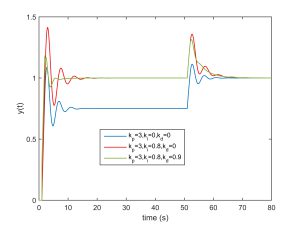
Fig. 12: Simulation results of PID manual tuning
Simulation Without Matlab/Simulink
If you don’t have access to Matlab/Simulink you can use the following websites for online simulation of the methods explained above.
- Simulator #1 (Features: online, unity feedback control system, PID controller in series with a first-order plus time delay – FOPTD – process in the forward path, simulation of the unit step setpoint tracking)
- Simulator #2 (Features: Excel tool to simulate a PID controller on a FOPTD process, open-loop and closed-loop simulations are possible)
You can find amazing films on tuning PID/PI controllers here.
Written by Farshad Merrikh Bayat, last updated on September 27, 2022